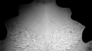
What if we want to visualize a change in refractive index that is gradual and/or not a large change? For example, we might visualize a region of heated air exhaled from a human, as shown in Figure 1. For this, shadowgraphy and schlieren are the techniques of choice. Both start with creating a beam of collimated light large enough to encompass the region of interest. Changes in refractive index then cause deflection of the collimated light, and an image of the region results. Generally these techniques are performed in air but they work in water and oil as well .
Shadowgraphy
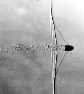
Caustics are a special case of a more general technique: shadowgraphy. Shadowgraphy can range from making the shadows of your hands look like rabbits to visualizing the shock wave and turbulent wake of a bullet in flight (Figure 2).
Light source
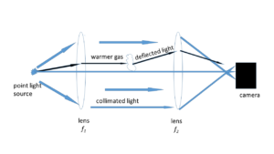
First you’ll need collimated light; parallel light with a circular cross section, like a column. This can be generated by the sun (parallel due to its extreme distance, but not perfect due to the sun’s diameter) or, as is more usual in a laboratory, by a point source at the focal point of a lens or concave mirror, as shown in Figure 3. The best point light source will be as small as possible and not too bright. Thirty years ago, the brightest possible sources were needed: films were not that sensitive, and typical subjects required very short shutter speeds, like in Figure 2. The challenge was finding a bright source with a small size. Today, in contrast, modern cameras are quite sensitive, and even very small LEDs can be too bright. 80 lumens is usually sufficient, and less than a 2-mm diameter LED is good. Be sure to use a high-quality, steady power supply to minimize flickering. Place the light source one focal length from your lens or concave mirror. You might be tempted to use a laser to generate the collimated light, but don’t! Laser light is also coherent; all the wave fronts are lined up, so they will interfere with each other strongly, both constructively and destructively, and the result will be a messy image. If you need to de-cohere laser light for some reason, try passing it through some milk.
Imaging
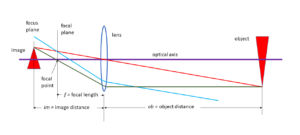
Now, why does this work? What exactly does the camera see? Let’s do a thought experiment. What will a camera (or your eye) see, looking at purely collimated light coming in along the optical axis, with the camera lens focused at infinity?
A. Uniform brightness
B. Single point of light
C. Small dot
D. Something else
Not sure? Here’s a hint: what natural light source do you know that emits collimated (parallel) light?
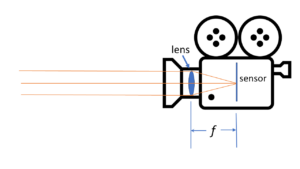
Hint Number 2: What do the lens laws say about light entering parallel to the optical axis? Single point of light. Like seeing a star. The light comes from so far away that it is quite parallel. When you focus on it, it resolves into a single point. Did you get it? When I ask this question in class, about 40% get it wrong. OK, let’s review the basic optics from back in the Overview. Here are the lens laws again: Consider an object very far away. Point the camera at it so the object is on the optical axis. The lens focus equation tells us that for large ob the image will be formed one focal length from the lens, so we want to place the sensor there for the object to be in focus. The object is far away, so the light from it is parallel, or nearly so, as shown above in Figure 4. The other lens laws tell us that all that parallel light will end up at one point on the sensor. Voila, an image of a point. OK, not very interesting from a flow vis point of view, but it illustrates what happens to parallel light entering a camera, or your eye. Turn the beams around, and it also illustrates why you place a point source at the focal point of a lens or mirror to get collimated light. Now let’s go back to the setup in Figure 2, with a second lens (focal length f2) that returns the collimated light into a point, and put that point one camera lens focal length (focal length f3) in front of our camera. What will the camera see now? A. Uniform brightness A. Uniform brightness.
B. Single point of light
C. Small dot
D. Something else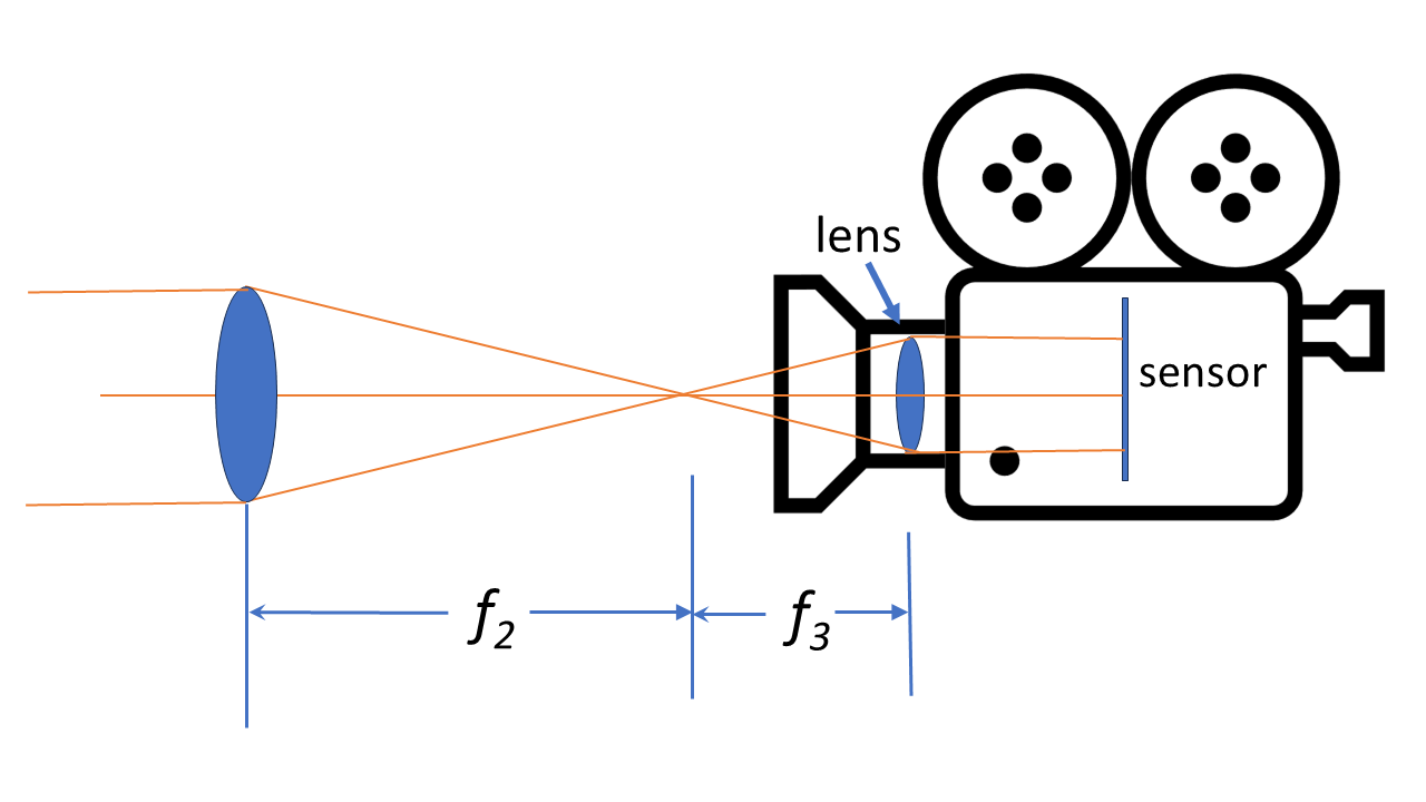
Next, let’s put something worth imaging in the collimated light. An easy test subject is something warm: a candle or a mug of hot water, perhaps. The mug will heat the air around it, reducing its density and index of refraction. The water vapor coming off the water will also have a different refractive index. The combined plumes will be irregular in shape, resulting in some of the collimated light being refracted — deflected. This refracted/deflected light will enter the second lens at a different angle than the rest of the column, and it won’t pass through the same focal point, although it will probably be close. The sensor won’t see a uniform brightness any more; some rays will be missing, and the refracted light will instead add brightness to other areas. The missing rays form a negative image of the plume: this is the shadowgraph. The deflected light rays end up elsewhere in the image where they can reduce the contrast of the image. This brings us to schlieren.
Schlieren
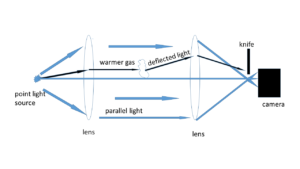
Schlieren uses the same setup, but goes one step further and cuts or filters the deflected light. This not only increases contrast but changes the physics to some degree. If you do the math, it turns out that schlieren is sensitive to gradients (first derivative) in index of refraction and shadowgraphy is sensitive to gradients in the gradients, i.e., 2nd derivative .
By the way, schlieren is a regular German noun that means, well, this effect. It comes from the German schliere, meaning “streak” . It’s not somebody’s name, so it doesn’t get capitalized in English except at the start of a sentence.
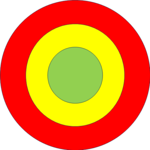
The easiest way to cut out the deflected light is literally with a knife or razor blade, as shown in Figure 7. This will show refractive index gradients in one direction and gives excellent contrast and sensitivity. There are many alternatives to this arrangement, which can highlight other gradients. For example, a circular iris, which blocks out all deflected light will show gradients in all directions. The reverse of this, a single opaque dot on a transparent slide will block out the un-deflected light, resulting in ‘dark-field schlieren.’ A color bulls-eye transparency, such as shown in Figure 8, can be used to color code the magnitude of the deflections: slight deflections are yellow, larger deflections are green, etc. This is known as ‘color schlieren.’
When you are setting up a schlieren system, it’s not so simple, of course. First, you won’t have a perfect point light source; it will have a finite size. Second, to get good collimated light over a large area — large enough to contain an interesting experiment — you need relatively long system focal lengths ( f1, f2). This is due to the economics of large optics; longer focal lengths mean less curvature at the edges — much easier to manufacture. Long focal lengths, for the linear system described so far, make the whole setup very difficult to fit in a room. Two strategies are commonly used to mitigate this problem: the Z-fold and the single mirror setup.
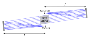
Figure 9 shows the Z-fold. This design has a number of benefits. It can be used with both parabolic and spherical mirrors. By using a matched pair of mirrors and identical small angles, it neatly cancels coma, an aberration caused by placing the source off axis of the first mirror . It is not sensitive to the distance between the mirrors, although more than 2f is needed in order to have a comfortable working area for the schlieren subject.
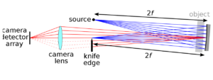
Figure 10 shows the single-mirror setup. Very handy, if you only have one mirror. Lens Law 4, the focus equation, tells us that for the source placed 2f from the lens you will form the image of the source at 2f also, where you can then apply the knife edge or target, allowing the rest of the light to continue and form the image in your camera. The test subject should be placed a short distance in front of the mirror. Be careful! Don’t let your test subject splash or spray or sneeze on your mirror; remember that first surface mirrors are fragile and almost impossible to clean safely. If you happen to have a beamsplitter, you can keep the source on the mirror’s axis and bounce the image off to the side on its return trip. Otherwise, keep the source as close to the knife edge as possible, but you will get some extra reflections of your subject and the schlieren in the image. This arrangement is indeed easier to setup and align than the Z-fold, but the schlieren quality is not as good, especially if you must put the source off-axis.
Both the schlieren and shadowgraph techniques are quick to give initial images. There are many Youtube videos showing how to set up DIY single-mirror systems, but really high quality images take painstaking alignment and high-quality equipment. If you are willing to invest the time and money, then Schlieren and Shadowgraph Techniques by Gary Settles is the must-have reference text. All the secrets to good schlieren are there. Prof. Settles tells me a second edition is on the way!
Background-Oriented Schlieren
Although schlieren and shadowgraphy have been around for almost two hundred years, modern computational power has enabled a very clever new variant. In the summer you have likely noticed road surfaces shimmer in the distance as hot air rises off the surface and distorts your view of the background. If you could get an image of the undisturbed background and compare it to the distorted view, you would see the same information that schlieren shows. This is basically how Background-Oriented Schlieren (BOS) works. Some fairly sophisticated image analysis is required to get the image and this is currently an active area of research , but there are a few open source software projects that you can play with .
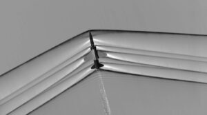
Generally this technique is performed in a laboratory with a printed pattern background, but NASA has performed this in open air to image aircraft shock waves, as shown in Figure 11. I thought the shadows in this photo were a little odd, until I read about the method and realized that the image is taken looking down on the aircraft; the ground forms the background. An empty photo of the ground is made, and then another is taken with the aircraft passing through. Post-processing removes the (back)ground and reveals the shock structure.

.jpg)